The Sharks of the Kelp Forest
Southern Africa’s kelp forests, particularly around the Cape Peninsula, harbor a remarkable diversity of shark species, some of which are found nowhere else on Earth. Along rocky reefs and sandy flats, these cryptic hunters will wriggle their way into your hearts with their mesmerising patterns, interesting hunting techniques, and endearing defense mechanisms.
The Shysharks
This genus of shark - Haploblepharus - are named for their charming defensive behaviour. When threatened, they curl into circles and cover their eyes with their tails. This genus includes four species: Puffadder shysharks, H. edwardsii, or “Happy Eddies”; Dark shysharks, H. pictus; Brown shysharks, H. fuscus; Natal shyshark, H. kristnasanyi (not included because they are data deficient on iNat). Shysharks are oviparous, laying eggs in tough capsules attached to rocks or kelp. They’re nocturnal hunters that rest during the day, often piled togethre in caves with their heads tucked in crevices.
The Poroderma Catsharks
The genus Poroderma includes two diver favourite sharks. Spotting their iconic patterns slipping through sea bamboo (Ecklonia maxima) is such a treat. The pyjama shark (P. africanum) is instantly recognisable by it’s bold dark striped over a light grey body and gained notoriety through “My Octopus Teacher” where it starred as the villain (as sharks often do). Similar to the shysharks, they can be found sleeping in the day piled on top of each other in cracks between rocks or nestled in dark corners of shipwrecks and old pipes. At night they emerge to hunt octopuses, lobsters, crabs, and fish. The leopard catshark (P. pantherinum) is the pyjama shark’s smaller, more elusive cousin sporting dark rosettes instead of striped (though some individuals’ rosettes merge to create dark streaks). Leopard catsharks are more cryptic, preferring tight cracks and crevices, making them harder to spot (pun intended).
The Izak Catsharks
Holohalaelurus (nicknamed hallelujah sharks) are deep-dwelling (100 - 400 m) catsharks characterised by broad, flattened heads and ornate patterns. The Izak catshark, H. regani, is the most abundant along the Southern African coastline. Despite being regularly caught as bycatch in hake trawl fisheries, populations have been increasing (rare among commercially impacted sharks). The African spotted catshark (white-spotted Izak), H. punctatus, is a small dwarf catshark that uses a unique sidewinding locomotory technique to capture prey. Unfortunately this species has suffered a dramatic decline, representing an estimated 50 to 79% population decline. The honeycomb Izak or Natal Izak, H. favus, hasn’t been seen since the mid-1970s despite intensive research efforts, suggesting it may be critically endangered or extinct. Unfortunately I had to leave these out of the maps as there were no observations on iNaturalist (c’mon fishermen - join the fun!).
Other Benthic Catsharks
The yellow-spotted catshark, Scyliorhinus capensis, is aptly named as it is covered in small golden-yellow spots over light grey and dark saddle patches. These nocturnal predators frequent rocky reefs and sandy bottoms but face pressure as bycatch in hake fisheries and are considered Near Threatened by the IUCN. The tiger catshark, Halaelurus natalensis, have dark dorsal saddles creating stripes resembling tigers - or so the people who named them say - and distinctive upturned snouts. They are endemic to Southern Africa, but face a population decline of 30 - 49% due to trawling pressure.
The Spotted Gully Shark
Also known as the sharptooth houndshark, Triakis megalopterus, have exceptionally long fins that provide stability and agility for maneuvering along the seafloor. They often form large aggregations during breeding seasons, particularly in False Bay. Despite their size (reaching up to 2 m), they fall prey to sevengill sharks and face vulnerability to overfishing and slow growth rates.
The Broadnose Sevengill Shark
These sharks, Notorynchus cepedianus, resemble ancient sharks (we’re talking older than trees here) and have a lineage dating back 1 million years (the mid-Pleistocene). Their old roots can be seen in the number of gill slits they have - 7 where most sharks have 5 - and their lacking dorsal fin. They hunt seals, fish, squids, rays, and other sharks and have been observed using cooperative hunting tactics. They are silver-grey to brown with scattered black and white spots, and can reach 3 m in length. Though once common in False Bay waters (especially around Miller’s Point), they are now a rare sight to see. The reason for their decline is uncertain but has been impacted - similarly to the white sharks - by the predation of Cape Town’s visiting orcas Port and Starboard (named for their floppy dorsal fins falling left and right respectively).
This is a distributional map of some cool sharks around the coast of Southern Africa (and the Southern Hemisphere - in the case of sevengill sharks).
Anywho - thank you for sticking with me through this! As a reward here’s a little picture of a shyshark I took a while back.
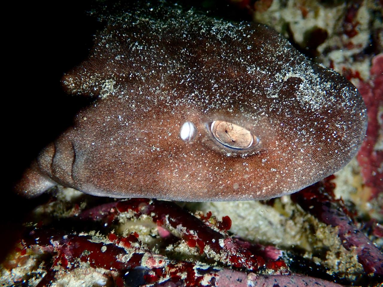
Happy Eddy - ‘Haploblepharus edwardsii’ - photographed at Windmill Beach, Cape Town.
Okay - SO LONG AND THANKS FOR ALL THE FISH!!
Thank you Jasper Slingsby for providing the base code for this. To access it go to his teaching website plantecolo.gy.